Plot RPA data

Show how we can exploit the signals from the Retarding Potential Analyzer/Retarding Field Analyzer.

Set up

Load some libraries

import tomllib
import pandas as pd
from pathlib import Path
from pprint import pprint

from multipac_testbench.instruments import RPACurrent, RPAPotential, RPA
from multipac_testbench.multipactor_test import MultipactorTest

Here is a sample of the TOML we will load, with some comments.

[global.instruments_kw.NI9205_ERPA]
caliber_mA = 20.0  # Caliber for the current data; used to rescale the measured signal
class_name = "RPACurrent"
# keyword arguments for the `average_y_for_nearby_x_within_distance` function
# it is used to average RPACurrent values measured at the same RPAPotential
average = true          # Activate averaging
keep_shape = true       # Recommended
max_index_distance = 1  # Averaging is performed on neighboring identical potential values.
                        # Increase it to like 1000 if you want to average over the whole tests
                        # (eg several power cycles)
tol = 1e-6

[global.instruments_kw.NI9205_Spellman]
class_name = "RPAPotential"

See also

Check the documentation of average_y_for_nearby_x_within_distance() for more information on the the averaging arguments.

project = Path("../data/campaign_ERPA")
config_path = Path(project, "testbench_configuration.toml")

with open(config_path, "rb") as f:
    config = tomllib.load(f)

results_path = Path(project, "MVE5-120MHz-50Ohm-BDTcomp-ERPA1_1dBm.csv")

Load data. Note that the info key will be appended to plots titles.

multipactor_test = MultipactorTest(results_path, config, freq_mhz=120.0, swr=1.0, sep=",", info="1dBm (175W)")

ERROR:root:Your Sample index column does not start at 0. I should patch this, but meanwhile expect some index mismatches.

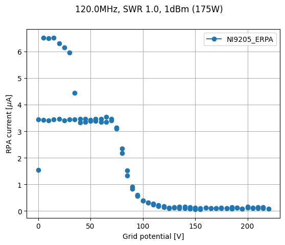
Plot collected current vs grid potential

In this test, RPA Current was measured twice at every potential. This is why we averaged it.

As we want to keep the shape of averaged data consistent with all the other instruments, we introduced NaN numbers for duplicated potential values.

rpa_potential = multipactor_test.get_instrument(RPAPotential)
rpa_potential_data = rpa_potential.data_as_pd.copy()
rpa_potential_data.name = "RPA potential [V]"

rpa_current = multipactor_test.get_instrument(RPACurrent)
rpa_current_data = rpa_current.data_as_pd.copy()
rpa_current_data.name = "Averaged RPA current [uA]"


resume_rpa = pd.concat([rpa_potential_data, rpa_current_data], axis=1)
display(resume_rpa[40:50])

	RPA potential [V]	Averaged RPA current [uA]
Sample index
41	5.0	6.518785
42	5.0	NaN
43	10.0	6.500730
44	10.0	NaN
45	15.0	6.513861
46	15.0	NaN
47	20.0	6.297208
48	20.0	NaN
49	25.0	6.154414
50	25.0	NaN

In the above table, you can see that the second measurement point at 5V is NaN. It is because the first measurement point is now a mean of both points.

The inconvenient is that plot lines are interrupted by these ``NaN`` values:

_, _ = multipactor_test.sweet_plot(
    RPACurrent,
    xdata=RPAPotential,
    marker="o",
)

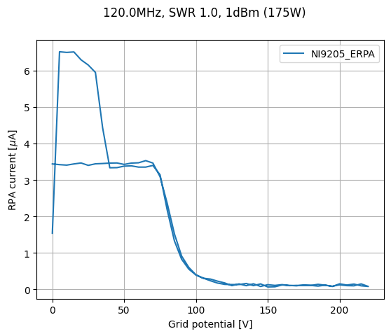
Use the drop_repeated_x argument to force the display of lines anyway.

_, _ = multipactor_test.sweet_plot(
    RPACurrent,
    xdata=RPAPotential,
    drop_repeated_x=True,
)

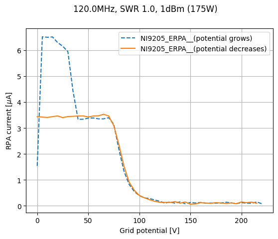
Tip for clearer plots

We start by calculating, for each measurement point, if potential was increased.

rpa_potential_growth_mask = rpa_potential.growth_mask(
    minimum_number_of_points=2, n_trailing_points_to_check=0
)

Now we set the masks dictionary. Remember that keys should start with double underscore (__).

masks = {
    "__(potential grows)": rpa_potential_growth_mask,
    "__(potential decreases)": ~rpa_potential_growth_mask,
}

And we are ready to plot!

_, _ = multipactor_test.sweet_plot(
    RPACurrent,
    xdata=RPAPotential,
    drop_repeated_x=True,
    masks=masks,
)

Plot energy distribution

The RPA object is automatically created when a RPACurrent and a RPAPotential are defined in the configuration TOML. It holds the electrons energy distribution, directly calculated from the RPA current and potential. To visualize it, you just need to:

rpa = multipactor_test.get_instrument(RPA)
axes = rpa.data_as_pd.plot(x=0, y=1, grid=True, xlabel="Electrons energy [eV]", ylabel="Distribution", title=str(multipactor_test))
_ = axes.set_ylim([-0.05, 0.35])

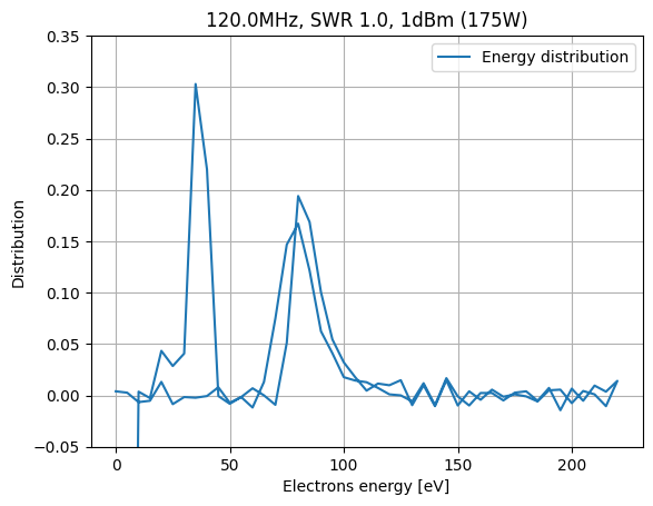
Currently, no dedicated method for this plot. Don’t know yet how I will implement this.

Todo

• Integrate to MultipactorTest.sweet_plot()? Maybe a dedicated method is more suited.

• Handle increasing/decreasing potentials to avoid superposition of the two distributions.