Plot signals measured by the instruments

This notebook showcases how basic plots of instrument signals can be produced.

Load data

Load libraries :

from multipac_testbench.multipactor_test import MultipactorTest
import multipac_testbench.instruments as ins

Set path to config and results files :

from multipac_testbench.data import config_path
from multipac_testbench.data.multipactor_tests import test_140MHz_SWR4_11

results_path = test_140MHz_SWR4_11

Note

In a real life example, results_path should be the path to a test file, CSV or XLSX. The simplest way to create one is through LabViewer.

Similarly, config_path should be the path to your test bench configuration file. See dedicated documentation

Now the MultipactorTest holding the test can be created with:

multipactor_test = MultipactorTest(results_path, config_path, freq_mhz=140., swr=4., sep=',', is_raw=True)

ERROR:root:column_header = 'NI9205_E1' not present in provided file. Skipping associated instrument.

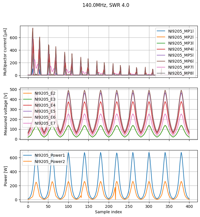
Plot signal measured by instruments

to_plot = (ins.CurrentProbe, ins.FieldProbe, ins.Power)
figsize = (8, 8)
_, _ = multipactor_test.sweet_plot(*to_plot, figsize=figsize)

Show all instruments that can be plotted

The full list of Instrument can be visualized with:

ins.__all__

['CurrentProbe',
 'IElectricField',
 'FieldPowerError',
 'FieldProbe',
 'ForwardPower',
 'Frequency',
 'Instrument',
 'OpticalFibre',
 'Penning',
 'Power',
 'PowerSetpoint',
 'Reconstructed',
 'ReflectedPower',
 'ReflectionCoefficient',
 'RPA',
 'RPACurrent',
 'RPAPotential',
 'SWR',
 'VirtualInstrument']